Chapter 4 Simulating population structure

A toy example for this Charpter can be found in gc5k’s Rpub

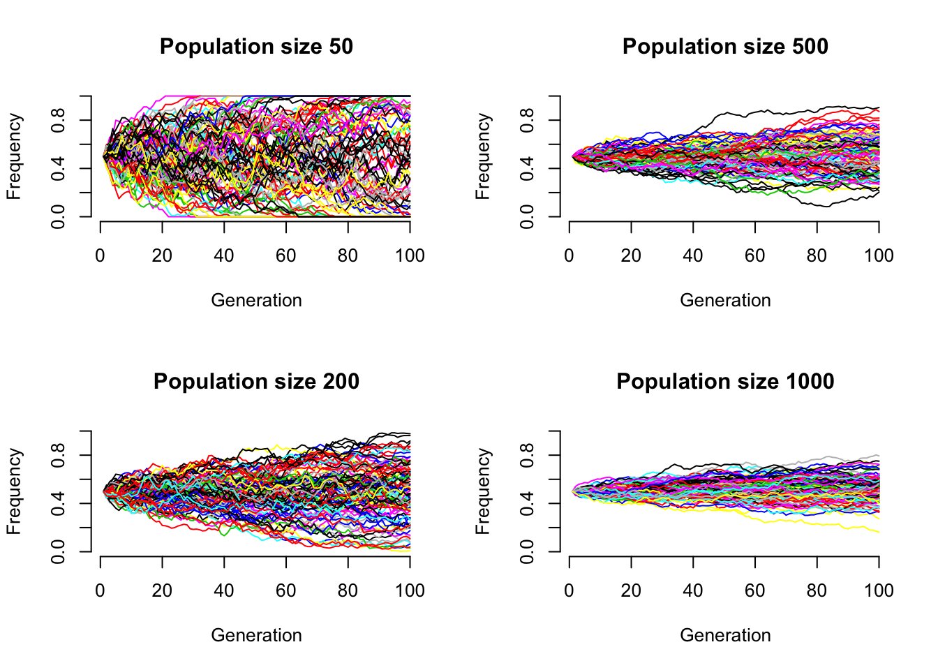
4.1 Genetic drift

As each locus follows binomial distribution, the genetic drift can be modelled \(\frac{\sqrt{pq}}{2n_e}\), in which \(n_e\) is the effective population size.

4.2 Discrete populations

Algorithm

Generate frequency \(f\) from the uniform distribution \((0.05, 0.95)\).
Given \(F_{st1}\), generating \(z_{1|1}\) and \(z_{2|1}\) from \(Beta(f\frac{1-F_{st1}}{F_{st1}}, (1-f)\frac{1-F_{st1}}{F_{st1}})\), respectively. The mean of them will be \(f\), and their sampling variance will be \(F_{st}\). Similarly, generate \(z_{1|2}\) and \(z_{2|2}\).
Set \(D_1\) and \(D_2\), the realized frequencies of the two populations.

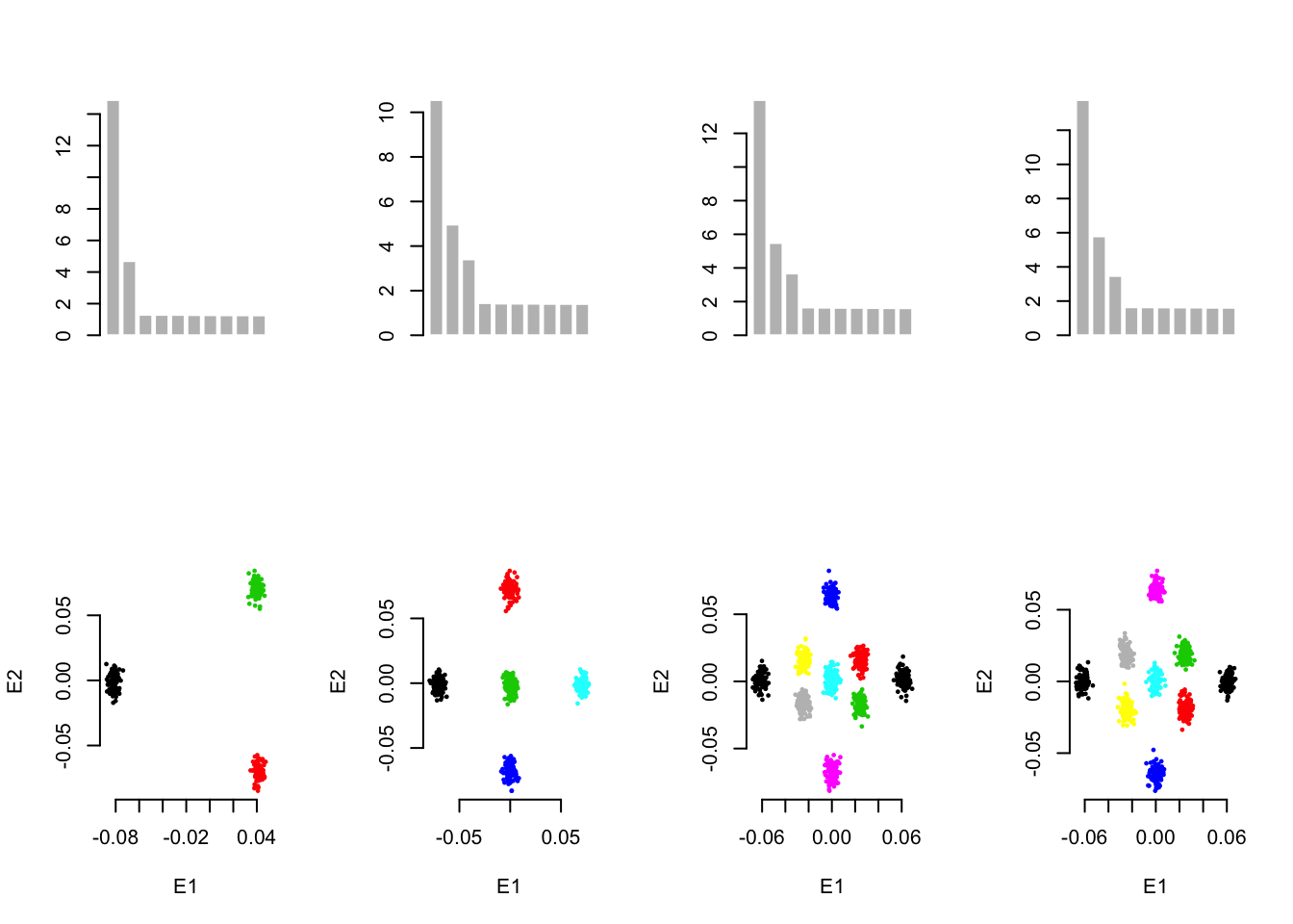
For the three-population simulation \[\begin{equation} F= \left ( \begin{array}{cc} 1 & 0\\ 0 & 1 \\ 0 & 1\\ \end{array} \right ) \left ( \begin{array}{c} z_{1|1}\\ z_{2|1}\\ \end{array} \right ) + \left ( \begin{array}{cc} 0 & 0\\ 1 & 0 \\ 0 & 1\\ \end{array} \right ) \left ( \begin{array}{c} z_{1|2}\\ z_{2|2}\\ \end{array} \right) \end{equation}\]

Below are three simulations generated from 3, 5, and 9 populations, each of which has 100 individuals; 10000 markers are used for each individual. \(D_1\) and \(D_2\) are printed for the three simulations below.

For the five-population simulation,

\[\begin{equation} F=\left ( \begin{array}{cc} 1 & 0 \\ 0.5 & 0.5 \\ 0.5 & 0.5 \\ 0.5 & 0.5 \\ 0 & 1\\ \end{array} \right ) \left ( \begin{array}{c} z_{1|1}\\ z_{2|1}\\ \end{array} \right ) + \left (\begin{array}{cc} 0 & 0 \\ 1 & 0 \\ 0 & 0 \\ 0 & 1 \\ 0 & 0\\ \end{array} \right) \left( \begin{array}{c} z_{1|2}\\ z_{2|2}\\ \end{array} \right) \end{equation}\]

For the nine-population simulation, scheme 1 \[\begin{equation} F=\left ( \begin{array}{cc} 1 & 0 \\ 0.3 & 0.7 \\ 0.3 & 0.7 \\ 0.5 & 0.5 \\ 0.5 & 0.5 \\ 0.5 & 0.5 \\ 0.7 & 0.3 \\ 0.7 & 0.3 \\ 0 & 1 \\ \end{array} \right) \left( \begin{array}{c} z_{1|1}\\ z_{2|1}\\ \end{array} \right) + \left ( \begin{array}{cc} 0 & 0 \\ 0.42 & 0.18 \\ 0.18 & 0.42 \\ 1 & 0 \\ 0 & 0 \\ 0 & 1 \\ 0.42 & 0.18 \\ 0.18 & 0.42 \\ 0 & 0 \\ \end{array} \right ) \left ( \begin{array}{c} z_{1|2}\\ z_{2|2}\\ \end{array} \right ) \end{equation}\]

For the nine-population simulation, scheme 2 \[\begin{equation} F=\left ( \begin{array}{cc} 1 & 0 \\ 0.3 & 0.7 \\ 0.3 & 0.7 \\ 0.5 & 0.5 \\ 0.5 & 0.5 \\ 0.5 & 0.5 \\ 0.7 & 0.3 \\ 0.7 & 0.3 \\ 0 & 1 \\ \end{array} \right) \left( \begin{array}{c} z_{1|1}\\ z_{2|1}\\ \end{array} \right) + \left ( \begin{array}{cc} 0 & 0 \\ 0.3 & 0.0 \\ 0.0 & 0.3 \\ 1 & 0 \\ 0 & 0 \\ 0 & 1 \\ 0.3 & 0.0 \\ 0.0 & 0.3 \\ 0 & 0 \\ \end{array} \right ) \left ( \begin{array}{c} z_{1|2}\\ z_{2|2}\\ \end{array} \right ) \end{equation}\]

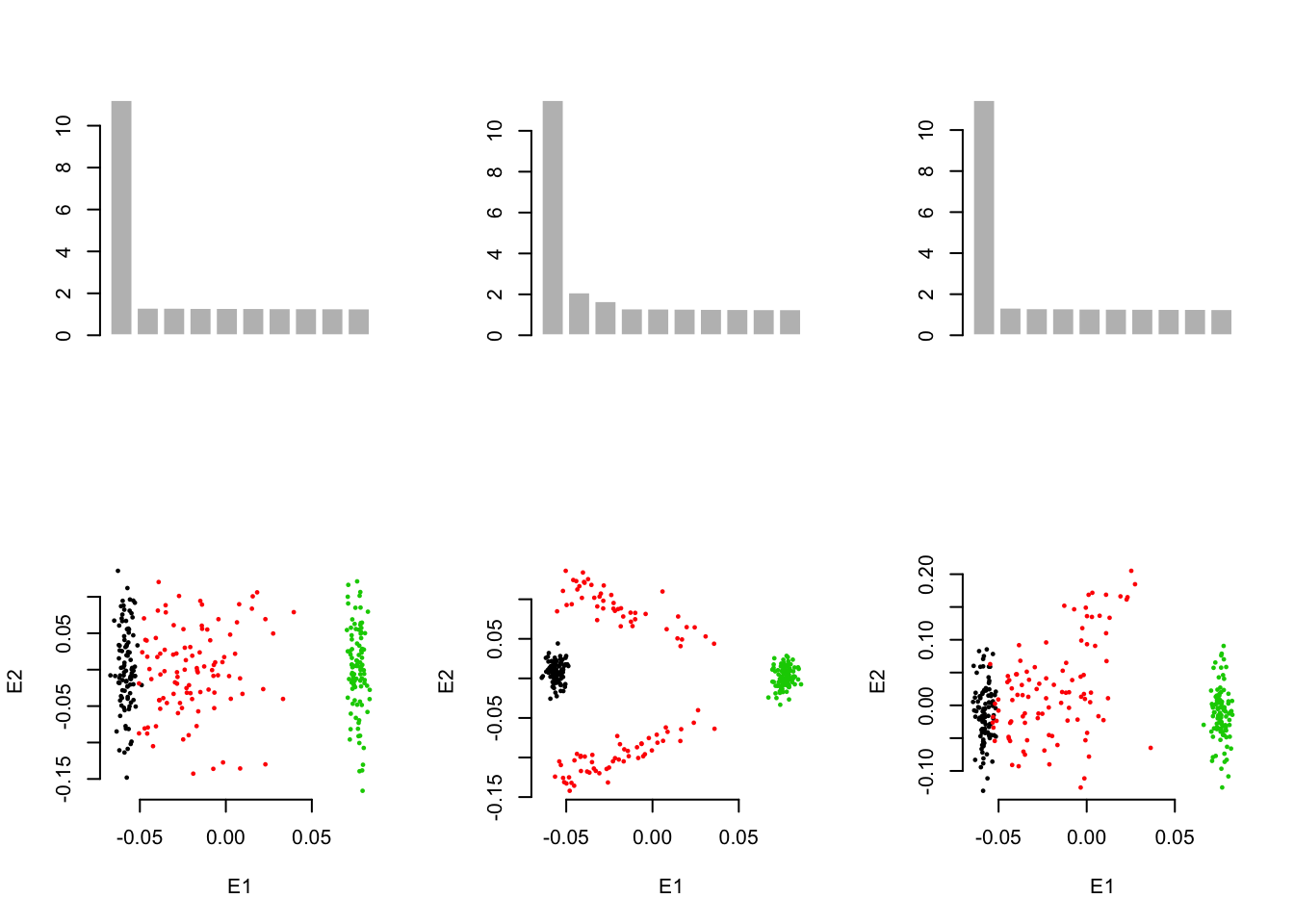
4.3 Admixture populations

4.4 Homo & Heteogeneous \(F_{st}\)

4.5 Wishart distribution

R function rWishart can generate Wishart distribution easiliy.

## Artificial
S <- toeplitz((10:1)/10)
set.seed(11)
R <- rWishart(1000, 20, S)
dim(R)  #  10 10  1000

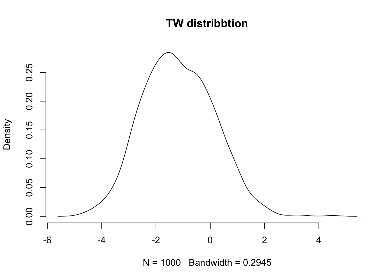
## [1]   10   10 1000

4.6 Tracy-Widom distribution

R package RMTstat can help study Tracy-Widom distribution.

library(RMTstat)
plot(density(rtw(1000)), main="TW distribbtion", bty='n')